Creating a Condition File Manually

To run RMG, you must specify the initial conditions and the model generation parameters, all of which are contained in a single file, condition.txt. The file condition.txt can be located in any directory, although it is advised that you create a special directory for RMG simulations, since each condition.txt creates its own subdirectories.

The condition.txt file should specify the following conditions, in order:

1. The main Database
2. Any restrictions on the number of atoms / radicals for all generated species
3. The name and location of all Primary Transport Libraries
4. The name and location of all Primary Thermodynamic Libraries
5. Optionally, some additional forbidden structures
6. The initial temperature and pressure of the system
7. The maximum number of carbons, oxygens, and radicals any one species may have
8. Whether to generate an IUPAC International Chemical Identifier (InChI) for each species
9. The name, concentration, and chemical structure of the reactants
10. The specification and concentration of the inert gas(es)
11. The method to use to estimate spectroscopic data for each species
12. The Pressure dependence model
13. The finish controller
14. The dynamic simulator
15. Sensitivity analysis settings
16. The name and location of all Primary Kinetic Libraries
17. The name and location of all Reaction Libraries
18. The name and location of all Seed Mechanisms
19. The units for the Arrhenius parameters A and Ea (to be reported in the generated chem.inp file)

The name condition.txt is variable. As you’ll see in Section Running RMG from the Command Line in Linux, you can change the name of the initialization file, so long as it remains a .txt file.

Database

In the main RMG directory is a directory of databases: $RMG/databases/. By default, there is one directory within the directory of databases: $RMG/databases/RMG_database. It is possible, however, to create multiple databases. For example, you can copy the entire contents of the default database into a new database, $RMG/databases/my_database, and change some of the values. Unless you have created your own databases, the Database setting should be left at the default value:

Database: RMG_database

Species Restrictions

By default, RMG will allow no more than 30 carbon atoms in any given species (other such default restrictions are: no more than 10 oxygen atoms, no more than 10 radicals, no more than 100 heavy-atoms, etc.). If you would like to change the default settings, the syntax is as follows

MaxCarbonNumberPerSpecies: 100
MaxOxygenNumberPerSpecies: 30
MaxRadicalNumberPerSpecies: 10
MaxSulfurNumberPerSpecies: 10
MaxSiliconNumberPerSpecies: 10
MaxHeavyAtomPerSpecies: 100

A “Heavy Atom” is defined in RMG as a non-hydrogen atom. Each of these fields is optional; the default values for all fields are listed here.

Changing the default values of these fields, in particular, lowering the maximum value per species, may help you if your simulations are running out of memory. Also, changing the default settings of these fields could be beneficial if you are only concerned with the decomposition of the initial species.

Primary Thermo Library

By default, RMG will calculate the thermodynamic properties of the species from Benson additivity formulas. In general, the group-additivity results are suitably accurate. However, if you would like to override the default settings, you may specify the thermodynamic properties of species in the primaryThermoLibrary. When a species is specified in the primaryThermoLibrary, RMG will automatically use those thermodynamic properties instead of generating them from Benson’s formulas. Multiple libraries may be created, if so desired. The order in which the primary thermo libraries are specified is important: If a species appears in multiple primary thermo libraries, the first instance will be used.

Please see Section Editing the Thermodynamic Database for details on editing the primary thermo library. In general, it is best to leave the PrimaryThermoLibrary set to its default value. In particular, the thermodynamic properties for H and H2 must be specified in one of the primary thermo libraries as they cannot be estimated by Benson’s method.

In addition to the default library, RMG comes with the thermodynamic properties of the species in the GRI-Mech 3.0 mechanism [GRIMech3.0].

[GRIMech3.0]

(1, 2) Gregory P. Smith, David M. Golden, Michael Frenklach, Nigel W. Moriarty, Boris Eiteneer, Mikhail Goldenberg, C. Thomas Bowman, Ronald K. Hanson, Soonho Song, William C. Gardiner, Jr., Vitali V. Lissianski, and Zhiwei Qin http://www.me.berkeley.edu/gri_mech/

This library is located in the $RMG/databases/RMG_database/thermo_libraries directory. All “Locations” for the PrimaryThermoLibrary field must be with respect to the $RMG/databases/RMG_database/thermo_libraries directory.:

PrimaryThermoLibrary:
Name: Default
Location: primaryThermoLibrary
Name: GRI-Mech 3.0
Location: GRI-Mech3.0
END

Primary Transport Library

By default, RMG will estiamte the transport properties (Lennard-Jones sigma and epsilon parameters) of a species from empirical correlations described by Tee et al. [Tee]; these correlations are functions of the acentric factor, the critical temperature, and the critical pressure. The acentric factor is estimated using the empirical correlation described by Lee et al. [Lee], which itself is a function of the critical pressure, the critical temperature, and the boiling temperature. The critical properties and boiling point are estimated using the Joback group-additivity scheme [Joback], [Reid].

[Tee]

L.S. Tee, S. Gotoh, and W.E. Stewart; “Molecular Parameters for Normal Fluids: The Lennard-Jones 12-6 Potential”; Ind. Eng. Chem., Fundamentals (1966), 5(3), 346-63 Table III: Correlation iii

[Lee]

B.I. Lee and M.G. Kesler; “A Generalized Thermodynamic Correlation Based on Three-Parameter Corresponding States”; AIChE J., (1975), 21(3), 510-527

[Reid]

R.C. Reid, J.M. Prausnitz and B.E. Poling; “The Properties of Gases and Liquids” 4th ed. McGraw-Hill, New York, NY, 1987

[Joback]

K.G. Joback; Master’s thesis, Chemical Engineering Department, Massachusetts Institute of Technology, Cambridge, MA, 1984

If you would like to override the default settings, you may specify the transport properties of species in the PrimaryTransportLibrary. Similar to the PrimaryThermoLibrary, RMG will automatically use those transport properties instead of estimating them using the methods described above. Multiple libraries may be created, if so desired. The order in which the primary transport libraries are specified is important: If a species appears in multiple primary transport libraries, the first instance will be used.

RMG comes with the transport properties of the species in the GRI-Mech 3.0 mechanism [GRIMech3.0]. This library is located in the $RMG/databases/RMG_database/transport_libraries directory. All “Locations” for the PrimaryTransportLibrary field must be with respect to the $RMG/databases/RMG_database/transport_libraries directory.

PrimaryTransportLibrary:
Name: GRI-Mech 3.0
Location: GRI-Mech3.0
END

Forbidden Structures

It is possible, though not necessary, to specify additional forbidden structures in the condition file. This section should appear after the PrimaryThermoLibrary section. Each adjacency list can be a species, as described in the Reactants section, but can contain wildcards as described in the Thermo Database and Adjacency List Notation section. For example:

ForbiddenStructures:
AdjacentBiradicalCs
1 C 1 {2,S}
2 C 1 {1,S}

AdjacentBiradicalCd
1 C 1 {2,D}
2 C 1 {1,D}

END

Note that each adjacency list must be followed by an empty line, and that the section must end (after an empty line) with the word END.

Initial Conditions

The next item in the initialization file is the initial temperature and pressure. Currently, RMG can only model constant temperature and pressure systems. Future versions will allow for variable temperature and pressure. Please note that the temperature and pressure must be accompanied by a unit (in parentheses). Suitable temperature units are: K, F, and C. Suitable pressure units are: atm, torr, pa, and bar. The following example assumes that the system begins at 600 Kelvin and 200 atmospheres:

TemperatureModel: Constant (K) 600
PressureModel: Constant (atm) 200

You may also list multiple temperature and pressure conditions, as the example below shows:

TemperatureModel: Constant (K) 600 700 800 900
PressureModel: Constant (atm) 1 200

For cases in which multiple temperatures and pressures are listed, the model generator will simulate the system (still using an isothermal, isobaric model) at all possible combinations of the specified temperatures and pressures. Thus, the resulting reaction mechanism will be valid (within the given error tolerances, estimates, and various other assumptions) at all the conditions specified. (Note, however, that reported concentrations in the Final_Model.txt output file will only correspond to the first T/P combination.)

Maximum Number of Atoms/Radicals Per Species

The next item in the initialization file allows the user to override the maximum number of carbons, oxygens, and/or radicals any species in the model may have. To override the default values, the syntax is:

MaxCarbonNumberPerSpecies: 20
MaxOxygenNumberPerSpecies: 6
MaxRadicalNumberPerSpecies: 3

If any of these fields are not present in the condition.txt file, RMG will use the default values.

InChI Generation

The next item in the initialization file is the InChI generation command. An InChI, or IUPAC International Chemical Identifier, is an unique species identifier, with the exception of differing electronic or spin states, developed by IUPAC and NIST. An example of an InChI string (which represents the species caffeine) is:

InChI=1/C8H10N4O2/c1-10-4-9-6-5(10)7(13)12(3)8(14)11(6)2/h4H,1-3H3

The InChI is composed of layers, separated by a forward-slash (/):

1. Chemical formula layer
2. Connectivity layer
3. Hydrogen layer
4. ...

For the current release, the InChIs are used as another way to represent a molecule. In future releases, the InChIs will link RMG with an online thermochemical database: PrIMe, or Process Informatics Model. The union will allow RMG to search for a community-recommended thermochemical data entry (e.g. Arrhenius parameters, NASA polynomials) before using estimation techniques.

If this field is turned on, the InChI for each species in the model is located in the RMG_Dictionary.txt file.

More information on the InChI project may be found at http://www.iupac.org/inchi/. More information on the PrIMe project may be found at http://primekinetics.org/

To enable the InChI generation, the item should read:

InChIGeneration: on

To disable the InChI generation, the item should read:

InChIGeneration: off

Reactants

The name, concentration, and structure of each reactant must be specified. For each reactant, the first line should include the reactant number (e.g. (1)), its name (e.g. C2O2), and it’s concentration with units (e.g. 4.09e-3 (mol/cm3)). Acceptable units for concentration are “mol/cm3”, “mol/m3”, and “mol/l”. Furthermore, RMG will not accept a species name that begins with a number.

The next line defines the reactant structure, described by an adjacency list. The RMG Viewer and Editor is a useful tool for generating adjacency lists. Please note that you may choose the simplified adjacency list in which the hydrogen atoms are omitted (shown below):

InitialStatus:

(1) CH3OH 4.09e-3 (mol/cm3)
1  C 0 {2,S}
2  O 0 {1,S}

(2) O2 1.1E-7 (mol/cm3)
1  O 1 {2,S}
2  O 1 {1,S}

END

Please note that the keyword END must be placed at the end of the InitialStatus section.

If one of the reactants is a resonance isomer, you only need to define one of the resonance structures, and RMG will automatically detect the others.

Represent molecular oxygen, O₂, as shown above. This is a deviation from versions of the RMG database prior to RMG 3.2. For more detail, please see this discussion on representing oxygen.

Inert Gases

Following InitialStatus, the initialization file specifies which inert gases, if any, are used. Currently RMG can handle four inert gases: N₂, Ne, He, and Ar. If one of the gases is not used, set the concentration to 0.0 (mol/cm3). If no bath gas is used, set all concentrations to zero. In the example below, there is no nitrogen, the neon and helium are omitted, and the argon concentration is 2.21E-6 (mol/cm3):

InertGas:
N2 0.0 (mol/cm3)
Ar 2.21E-6 (mol/cm3)
END

To create valid CHEMKIN files, ensure that any 3rd-body collider molecules used in your Seed Mechanisms or Primary Reaction Libraries are either declared in their species.txt files (if they are reactive) or in this section. (i.e. it’s a good idea to list all of N2, Ne, He and Ar, even if their concentrations are 0)

Please note that the keyword END must be placed at the end of the InertGas section.

Spectroscopic Data

The next item in the initialization file is the method to use to estimate the spectroscopic data (i.e. rovibrational modes) of each species. At present there is only one method available, which utilizes approximate frequencies based on functional groups in the molecule when possible, then fits remaining degrees of freedom to heat capacity data. This can also be set to off if spectroscopic data is not needed (i.e. when pressure dependence is off).

When pressure dependent calculations are not desired, this item should read:

SpectroscopicDataEstimator: off

When pressure dependent calculations are desired, this item should read:

SpectroscopicDataEstimator: FrequencyGroups

Pressure Dependence

This flag is used to specify whether the model should account for pressure dependent rate coefficients. If pressure dependence is not desired, this item should read:

PressureDependence: off

If pressure dependence is desired, this item can take one of two values, based on the method used to approximate the pressure-dependent kinetics: ModifiedStrongCollision and ReservoirState. The former utilizes the modified strong collision approach of Chang, Bozzelli, and Dean [Chang2000], and works reasonably well while running more rapidly. The latter utilizes the steady-state/reservoir-state approach of Green and Bhatti [Green2007], and is more theoretically sound but more expensive.

To specify the modified strong collision approach, this item should read:

PressureDependence: ModifiedStrongCollision

To specify the reservoir state approach, this item should read:

PressureDependence: ReservoirState

For more information on the two methods, consult the following resources:

[Chang2000]

A.Y. Chang, J.W. Bozzelli, and A. M. Dean. “Kinetic Analysis of Complex Chemical Activation and Unimolecular Dissociation Reactions using QRRK Theory and the Modified Strong Collision Approximation.” Z. Phys. Chem. 214 (11), p. 1533-1568 (2000).

[Green2007]

N.J.B. Green and Z.A. Bhatti. “Steady-State Master Equation Methods.” Phys. Chem. Chem. Phys. 9, p. 4275-4290 (2007).

When pressure dependence is on, you must also specify a linear interpolation model to use to evaluate and output to the Chemkin file. (This line is not required if pressure dependence is set to off.) This line must immediately follow the previous one.

To disregard all temperature and pressure dependence and simply output the rate at the provided temperature and pressure, use the line

PDepKineticsModel: Rate

To use logarithmic interpolation of pressure and Arrhenius interpolation for temperature, use the line

PDepKineticsModel: PDepArrhenius

The auxillary information printed to the Chemkin chem.inp file will have the “PLOG” format. Refer to Section 3.5.3 of the CHEMKIN_Input.pdf document and/or Section 3.6.3 of the CHEMKIN_Theory.pdf document. These files are part of the CHEMKIN manual.

To fit a set of Chebyshev polynomials on inverse temperature and logarithmic pressure axes mapped to [-1,1], use the line

PDepKineticsModel: Chebyshev

You should also specify the number of temperature and pressure basis functions by adding the appropriate integers. For example, the following specifies that five basis functions in temperature and four in pressure should be used

PDepKineticsModel: Chebyshev 5 4

The auxillary information printed to the Chemkin chem.inp file will have the “CHEB” format. Refer to Section 3.5.3 of the CHEMKIN_Input.pdf document and/or Section 3.6.4 of the CHEMKIN_Theory.pdf document.

To generate the interpolation model, a set of temperatures and pressures must be used. RMG can do this automatically, but it must be told a few parameters. Following the previous line, you should provide a line to specify the minimum and maximum temperature and number of temperatures to use in the grid, e.g.

TRange: (K) 300.0 2000.0 8

A similar line should follow for pressures:

PRange: (bar) 0.01 100.0 5

If you prefer, you can also specify the grid of temperatures and pressures manually using lines similar to the following:

Temperatures: 8 (K) 300.0 400.0 500.0 600.0 800.0 1000.0 1500.0 2000.0
Pressures: 5 (bar) 0.01 0.1 1.0 10.0 100.0

You should specify either a TRange or Temperatures line and either a PRange or Pressures line.

Finish Controller

The Finish Controller defines the termination rules for model growth. Additionally, it includes the precision parameters such as reaction time, conversion, and error tolerance. The finish controller item should begin with a line that contains only FinishController:.

Below the Finish Controller line, you must specify the goal. The goal tells the program when to terminate the reaction model expansion. There are two goal options: ReactionTime and Conversion. ReactionTime must be followed by a number and a time unit. Acceptable units of time are “sec”, “min”, “hr”, and “day”. Conversion must be followed by a reactant species name and a number between 0 and 1.

Beneath the goal, you must specify the error tolerance. Typical values for the error tolerance are between 0.0001 and 0.5. A smaller error tolerance generally corresponds to a larger model and longer model generation times. In the first example, the reaction will run for 0.001 seconds:

FinishController:
(1) Goal ReactionTime: 0.001 (sec)
(2) Error Tolerance: 0.1

In the second example, the reaction will run until 90% of the C₂H₆ reactant is consumed and has a much tighter error tolerance:

FinishController:
(1) Goal Conversion: C2H6 0.90
(2) Error Tolerance: 0.0001

For the initial model run, it is often preferable to use Goal Conversion instead of Goal ReactionTime, since it is difficult to judge a priori what the reaction time should be.

For a more detailed description on rate-based model enlargement, please consult [Susnow1997].

Dynamic Simulator

RMG uses the DASSL or DASPK dynamic solver. DASSL is recommended, as RMG uses DASPK in a way that requires the use of the proprietary DAEPACK library, which is not distributed with RMG. Future versions of RMG might include the CHEMKIN dynamic solver.

The first line beneath the solver should be either TimeStep or Conversions, depending on whether you chose Goal Conversion or Goal ReactionTime as your finish controller criterion.

The TimeStep indicates at what time steps RMG should check to see if the model needs to be enlarged. By default the units of time steps is always seconds. For example in the example shown below RMG will stop at 0.0001 sec, 0.0002 sec ... and so on to see whether the error tolerance is satisfied:

DynamicSimulator: DASSL
TimeStep: 0.0001 0.0002 0.0004 0.0006 0.0008 0.0009

The other option is to specifiy the Conversions. In this option the conversion of the FinishController species (in this case, C₂H₆) is monitored and RMG will stop at conversions of 0.1, 0.2, ... and so on to see whether the error tolerance is satisfied:

DynamicSimulator: DASSL
Conversions: 0.1 0.2 0.4 0.6 0.8 0.9

For both TimeStep or Conversions, in addition to determining when RMG will stop to check whether error tolerances are satisfied, the concentrations and flux at the points specified will be reported in the Final_Model.txt file.

If you would not like to specify time steps or conversions, you may have them determined using the “automated time stepping” feature by specifying AUTO as follows:

DynamicSimulator: DASSL
TimeStep: AUTO

or:

DynamicSimulator: DASSL
Conversions: AUTO

The automated time stepping feature is described in greater detail in the Theory and Implementation Details appendix. When using automated time stepping, it is also possible to perform mechanism generation with pruning of “unimportant” edge species to reduce memory usage. This option is requested by specifying AUTOPRUNE in place of AUTO. When using AUTOPRUNE, this must be followed by four lines specifying pruning parameters, as the example below shows:

TerminationTolerance: 1.0E4
PruningTolerance: 1.0E-15
MinSpeciesForPruning: 1000
MaxEdgeSpeciesAfterPruning: 1000

TerminationTolerance and PruningTolerance are compared with the same quantity as Error Tolerance in the FinishController section (i.e. they are all compared with ratios of edge species flux to characteristic reaction model flux). TerminationTolerance indicates how high the edge flux ratio must get to interrupt the simulation (before reaching the Goal Conversion or Goal ReactionTime described earlier). Pruning won’t occur if the simulation is interrupted before reaching the goal criteria, so set this high to increase pruning opportunities. The value should be greater than or equal to Error Tolerance. PruningTolerance indicates how low the edge flux ratio for a species must get before the species is pruned (removed) from the edge (regardless of edge size relative to MaxEdgeSpeciesAfterPruning). The value should be (significantly) lower than Error Tolerance. MinSpeciesForPruning indicates the minimum total number of species (edge and core) that must be present for pruning (due to low edge flux ratio relative to PruningTolerance or due to MaxEdgeSpeciesAfterPruning) to occur. MaxEdgeSpeciesAfterPruning indicates the upper limit for the size of the edge. Pruning will continue until the edge is at least this small, regardless of PruningTolerance (though lowest fluxes are pruned first).

When using pruning, RMG will not prune unless all reaction systems reach the goal reaction time or conversion without first exceeding the termination tolerance. Therefore, you may find that RMG is not pruning even though the model edge size exceeds MaxEdgeSpeciesAfterPruning. In order to increase the likelihood of pruning in such cases, you can try increasing TerminationTolerance to an arbitrarily high value. Alternatively, if you are using a conversion goal, because reaction systems may reach equilibrium below the goal conversion, it may be helpful to reduce the goal conversion or switch to a goal reaction time.

The next two lines specify the absolute and relative tolerance for the ODE solver, respectively. Common values for the absolute tolerance are 1e-15 to 1e-25. Relative tolerance is usually 1e-4 to 1e-8:

Atol: 1e-20
Rtol: 1e-4

Note: You have the option of using sensitivity analysis only if you have the DASPK solver and the DAEPACK library. If you are using DASSL solver then skip the Sensitivity Analysis section.

One option when dealing with NegativeConcentrationException issues is to use the “non-negative” option with DASSL. This option is requested with the line “DynamicSimulator: DASSL: non-negative”. See the FAQ for further details.

Sensitivity Analysis

As long as DASPK is chosen for the dynamic solver, RMG can perform sensitivity analysis and generate error bars on the concentration profiles. As mentioned above, however, RMG uses DASPK in a way that requires the use of the proprietary library DAEPACK (which provides automatic differentiation capabilities for the sensitivity analysis). If you do not have access to this library, an alternative is to perform sensitivity analysis in CHEMKIN, using the ‘’chem.inp’’ file produced by RMG.

The sensitivity analysis is based upon first-order sensitivity coefficients and uncertainties in the rate constants. To use the sensitivity analysis, either the first or second line must be set to on. If both Error bars and Display sensitivity coefficients are set to off, then RMG will not perform a sensitivity analysis.

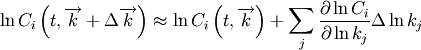
When the option to generate error bars is turned on, RMG calculates the upper and lower bounds on the concentration profiles for all core species. These upper and lower bounds are generated by the first-order sensitivity equation:

where is the concentration of the species, and is the vector of rate constants.

If the option to display sensitivity coefficients is turned on, you must specify a list of species for which the sensitivities should be displayed. The output file will then include the sensitivities of those species with respect to all the rate constants, all the heats of formations, and the initial concentrations of all the reactants. Additionally, if you choose to display the sensitivity coefficients, RMG will print a list of the five reactions that contribute the most to the uncertainty in the concentration (for each species selected by the user).

Sensitivities to rate constants are normalized sensitivities (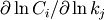), and sensitivities to heats of formation are semi-normalized (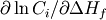). The contribution of a reaction to the uncertainty is estimated as the product of the normalized sensitivity and the uncertainty in the rate constant (). In the following example, RMG will perform a sensitivity analysis. Error bars will be generated for all the species, and the sensitivity coefficients will be generated for carbon monoxide, carbon dioxide, methane, and water:

Error bars: On
Display sensitivity coefficients: On
Display sensitivity information for:
CO
CO2
CH4
H2O
END

Please note that the keyword END must be placed at the end of the Error bars section.

Primary Kinetic Library

The next section of the condition.txt file specifies which, if any, primary kinetic libraries should be used. When a reaction is specified in a primary kinetic library, RMG will use these kinetics instead of the kinetics located in the RMG_database/kinetics_groups/<RxnFamily>/rateLibrary.txt directory.

For details of the kinetics libraries included with RMG that can be used as a primary kinetic library, see Kinetics Libraries. You can specify your own primary kinetic library in the location section. In the following example, the user has created her own primary kinetic library with a few additional reactions specific to n-butane, and these reactions are to be used in addition to the Leeds’ oxidation library:

PrimaryKineticLibrary:
Name: nbutane
Location: nbutane
Name: Leeds
Location: combustion_core/version5
END

If a user wished to use the GRI-Mech 3.0 mechanism as a primary kinetic library, the syntax is:

Name: GRI-Mech 3.0
Location: GRI-Mech3.0

The libraries are stored in $RMG/databases/RMG_database/kinetics_libraries/ and the Location: should be specified relative to this path.

Please note that the keyword END must be placed at the end of the Primary Kinetic Library section. Because the units for the Arrhenius parameters are given in each library, the different libraries can have different units.

If the same reaction occurs more than once in the combined library, the instance of it from the first library in which it appears is the one that gets used.

Changed in version 3.2: In previous versions this feature was called “PrimaryReactionLibrary” it has been renamed to “PrimaryKineticLibrary” to better represent its functionality.

Reaction Library

The next section of the condition.txt file specifies which, if any, Reaction Library should be used. When a reaction library is specified, RMG will first use the reaction library to generate all the relevant reactions for the species in the core before going through the reaction templates. This feature can be used as a Primary Kinetic Library and in addition also use to specify those reactions which the user wants to consider while building the mechanism but do not match any of RMG templates. In Reaction Library unlike the seed mechanism these reactions do not need to be included in the core from the start.

For details of the kinetics libraries included with RMG that can be used as a reaction library, see Kinetics Libraries. You can specify your own reaction library in the location section. In the following example, the user has created a reaction library with a few additional reactions specific to n-butane, and these reactions are to be used in addition to the Glarborg C3 library:

ReactionLibrary:
Name: nbutane
Location: nbutane
Name: Glarborg
Location: Glarborg/C3
END

The reaction library are stored in $RMG/databases/RMG_database/kinetics_libraries/ and the Location: should be specified relative to this path.

Please note that the keyword END must be placed at the end of the Reaction Library section. Because the units for the Arrhenius parameters are given in each mechanism, the different mechanisms can have different units.

Note

While using a Reaction Library the user must be careful enough to provide all instances of a particular reaction in the library file, as RMG will ignore all reactions generated by its templates.

In case the user has specified a reaction as only irreversible RMG will ignore all instances it generates even if they are reversible.

Seed Mechanisms

The next section of the condition.txt file specifies which, if any, Seed Mechanisms should be used. If a seed mechanism is passed to RMG, every species and reaction present in the mechanism will be placed into the core, in addition to the species that are listed in the Reactants section.

For details of the kinetics libraries included with RMG that can be used as a seed mechanism, see Kinetics Libraries.

You can specify your own seed mechanism in the location section. Please note that the oxidation library should not be used for pyrolysis models. The syntax for the seed mechanisms is similar to that of the primary reaction libraries, except for the GenerateReactions line, explained below.:

SeedMechanism:
Name: GRI-Mech 3.0
Location: GRI-Mech3.0
GenerateReactions: yes
Name: Leeds
Location: combustion_core/version5
GenerateReactions: yes
END

The seed mechanisms are stored in $RMG/databases/RMG_database/kinetics_libraries/ and the Location: should be specified relative to this path.

There is a new required GenerateReactions line in seed mechanisms that controls how RMG adds the seed species and reactions to the model core. If set to yes, RMG will use its reaction families to react all seed species with one another; the generated reactions will supplement the seed reactions. If set to no, RMG will not generate reactions of the seed species. In either case, RMG will react the species in the condition file with one another and with all species in the seed mechanism.

Please note that the keyword END must be placed at the end of the Seed Mechanism section. Because the units for the Arrhenius parameters are given in each mechanism, the different mechanisms can have different units. Additionally, if the same reaction occurs more than once in the combined mechanism, the instance of it from the first mechanism in which it appears is the one that gets used.

Note

For more information on what files to include in a Primary Kinetic / Reaction Library or Seed Mechanism, visit Building a Primary Kinetc Library / Reaction Library / Seed Mechanism

Chemkin Units

The last section of the condition.txt file specifies the units for the Arrhenius A and Ea parameters reported in the chem.inp file. The acceptable units for A are “moles” and “molecules”; the acceptable units for Ea are “kcal/mol”, “cal/mol”, “kJ/mol”, “J/mol”, and “Kelvins”:

ChemkinUnits:
A: moles
Ea: kcal/mol

Another option available to the user is to specify whether the comments following each set of Arrhenius parameters in the chem.inp file are concise or verbose. The verbose comments describe how the reported A, n, and Ea Arrhenius parameters were calculated in the event RMG could not find an exact match for the functional groups.:

ChemkinUnits:
Verbose: on
A: moles
Ea: kcal/mol

If the Verbose field is not present, RMG will default to “off”.

Note

The chem.inp file generated with the Verbose field turned “on” may have a comment that spans hundreds of characters. These verbose comments may cause the CHEMKIN interpreter to throw an error when running the Pre-Processor.